Bias-Varaince and Error Analysis
A Chinese version of this section is available. It can be found here. The Chinese version will be synced periodically with English version. If the page is not working, you can check out a back-up link here.
In this section, we focus on how bias and varaince are correlated. We always want to have zero bias and zero variance. However, this is practically impossible. So there is tradeoff in between.
1 The Bias-Varaince Tradeoff
Let’s denote $\overset{\wedge}{f}$ be the model that is trained on some dataset and $y$ be the ground truth. Then, the mean squared error(MSE) is defined:
\[\mathbb{E}_{(x,y)\sim \text{test set}} \lvert \overset{\wedge}{f}(x) - y \rvert^2\]We have three explanation for a high MSE:
Overfitting: The model does not generalize well and probably only works well in training dataset.
Underfitting: The model does not train enough or have enough data for training so does not learn a good representation.
Neither: The noise of data is too high.
We formulate these into Bias-Varaince Tradeoff.
Assume that samples are sampled from similar distribution which can be defined as:
$y_i = f(x_i) + \epsilon_i$ where the noise $\mathbb{E}[\epsilon] = 0$ and $Var(\epsilon) = \sigma^2$.
Whereas our goal is to compute f, we can only obtain an estimate by looking at training samples generated from above distribution. Thus, $\overset{\wedge}{f}(x_i)$ is random since it depends on $\epsilon_i$ which is random and it is also the prediction of $y = f(x_i) + \epsilon_i$. Thus, it makes sense to get $\mathbb{E}(\overset{\wedge}{f}(x)-y)$.
We can now calculate the expected MSE:
\[\begin{align} \mathbb{E}[(y-\overset{\wedge}{f}(x))^2] &= \mathbb{E}[y^2 + (\overset{\wedge}{f})^2 - 2y\overset{\wedge}{f}]\\ &= \mathbb{E}{y^2} + E[(\overset{\wedge}{f})^2] - \mathbb{E}[2y\overset{\wedge}{f}] \\ &= Var(y) + Var(\overset{\wedge}{f}) + (f^2 - 2f\mathbb{E}[\overset{\wedge}{f}] + (\mathbb{E}[\overset{\wedge}{f}])^2\\ &= Var(y) + Var(\overset{\wedge}{f}) + (f - \mathbb{E}[\overset{\wedge}{f}])^2\\ &=\sigma^2 + \text{Bias}(f)^2+ Var(\overset{\wedge}{f}) \end{align}\]The fisrt term is data noise which we cannot do anything. A high bias term means the model does not learn efficiently and is underfitting. A high variance means that the model does not generalize well and is overfitting.
2 Error Analysis
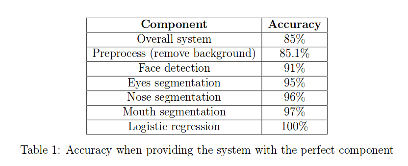
To analyze a model, we should first build a pipeline of the interests. Then, we start from plugging ground truth for each component and see how much accuracy that change makes on the model. We always try to see which componenet in ground truth is affect the most when adding to the system. An example can be seen below.
3 Ablative Analysis
Whereas error analysis tries to recognize the difference between current performance and perfect performance, Ablative Analysis tries to recognize that between baseline and current model. Ablation analysis is quite important, many research papers are rejected because of the missing of this part. This analysis can tell us which part of the model affects the most.
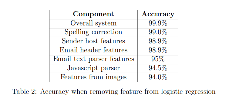
For example, assume that we have more add-on features that makes the model perform better. We want to see how much performance it will be reduced by eliminating one add-on feature at a time. An example can be shown below.