Ensembling Methods
Introduction
In Decision Tree section, we talked about how decision tree is applied in regression and classification task and how we can grow a decision tree. However, as also mentioned in the section, decision tree has limited power to generalize well. Thus, it has been proposed to use ensembling methods. In a word, multiple trained models perform better than the single model. But why?
Let’s have n i.i.d. random variables $X_i$ for $0 \leq i \leq n$ and assume $Var(X_i) = \sigma^2$ for all $X_i$. Then, we have the variance of the mean:
\[Var(\bar{X}) = Var(\frac{1}{n}\sum\limits_i X_i) = \frac{\sigma^2}{n}\]If we remove the independent assumption, then each random variable is correlated.
\[\begin{align} Var(\bar{X})&=Var(\frac{1}{n}\sum\limits_i X_i) \\ &= \frac{1}{n^2}\sum\limits_{i,j}Cov(X_i,X_j) \\ &= \frac{n\sigma^2}{n^2} + \frac{n(n-1)p\sigma^2}{n^2} \\ & = p\sigma^2 + \frac{1-p}{n}\sigma^2 \end{align}\]where p is pearson correlation coefficient $p_{X,Y} = \frac{Cov(X,Y)}{\sigma_x\sigma_y}$. We know that Cov(X,X) = Var(X).
Math: The following proof might be helpful for understanding the steps above.
\[\begin{align} Var(\frac{1}{n}\sum\limits_i X_i) &= \frac{1}{n^2} Var(\sum\limits_i X_i) \\ &= \mathbb{E}[(\sum\limits_i X_i)^2] - (\mathbb{E}[\sum\limits_i X_i])^2 \\ &=\mathbb{E}[\sum\limits_{i,j}X_i X_j] - (\mathbb{E}[\sum\limits_i X_i])^2 \\ &=\sum\limits_{i,j}\mathbb{E}[X_iX_j]- (\mathbb{E}[\sum\limits_i X_i])^2 \\ &= \sum\limits_{i,j}\mathbb{E}[X_iX_j] - \sum\limits_{i,j}\mathbb{E}[X_i] \mathbb{E}[X_j] \\ &= \sum\limits_{i,j} \mathbb{E}[X_iX_j] - \mathbb{E}[X_i] \mathbb{E}[X_j] \\ &= \sum\limits_{i,j} Cov(X_i,X_j) \end{align}\]Back to topic: Now, if we treat each random variable is the error of a trained model, we can see that the variance can be reduced by:
1, increase the number of random variable (i.e. number of models) n to make the second term smaller
2, reduce the correlation between each random variable to make the first term smaller, and it become more i.i.d.
How do we achieve those? Here, we will introduce Bagging and Boosting.
Bagging
Bootstrap
Bootstrap is basically a re-sampling technique for improving estimators on the data. In this algorithm, we keep sampling from the empirical distribution of the data to estimate statistics of the data.
Let’s say we have an trained estimator E for the statistic such as median of the data. The question is how confident our estimator is and how much variance it is. We can use bootstrap to find out. In bootstrap algorithm, we do:
1, Generate bootstrap samples $\mathbb{B}_1,\dots,\mathbb{B}_B$ where $\mathbb{B}_b$ is created by picking n samples from the dataset of size n with replacement
2, Evaluate the estimator on each $\mathbb{B}_b$ as:
\[E_b = E(\mathbb{B}_b)\]3, Estimate the mean and variance of E:
\[\mu_B = \frac{1}{B}\sum\limits_{n=1}^B E_b, \sigma_B^2 = \frac{1}{B}\sum\limits_{b=1}^B (E_b - \mu_B)^2\]This can tell us how our estimator performs on estimating the median of the data.
Bagging
Bagging basically uses the idea of bootstrap for regression or Classification. It represents Bootstrap aggregation.
The algorithm is as the following:
For $b=1,\dots,B$,
1, Draw a bootstrap $\mathbb{B}_b$ of size n from training dataset
2, Train a tree classifier or tree regression model $f_b$ on $\mathbb{B}_b$.
To predict, for a new point $x_0$, we compute:
\[f(x_0) = \frac{1}{B} \sum\limits_{b=1}^B f_b(x_0)\]For regression problem, we can see this is just the average of of prediction of each trained classifier. For classification task, we can use a voting mechanism for the final result.
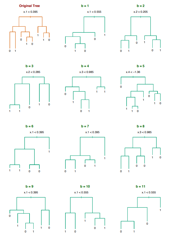
For example, let’s say we have an input feature $x\in \mathbb{R}^5$ for a binary classification. We can use bootstrap strategy to train multiple classifier as:
Let’s back to the equation:
\[Var(\bar{X}) = p\sigma^2 + \frac{1-p}{n}\sigma^2\]As we talked about, one way to reduce the variance is that we have less correlation on each trained model. Bagging achieves this by training on different datasets. One might concert about the fact that this will increase the bias since each bootstrap does not take the full training samples from the original dataset. However, it turns out that the decrease in variance is more than the increase in bias. Also, we can keep reducing variance by introducing more models (i.e. increase M or n in the equation). This will not lead to overfitting because $p$ is insensitive to M. Thus, overall variance can only decrease.
However, there are two key points that should be emphasized:
1, With bagging,each tree does not need to be perfect. “Ok” is fine.
2, Bagging often improves when the function is non-linear.
Out-of-bag estimation
In each bootstrap, we can only contain a portion of original dataset. Let’s assume that we sample it from uniform distribution with replacement. As dataset size $n\rightarrow \infty$, we have the probability of a sample not being selected as:
\[\begin{align} \lim\limits_{n\rightarrow \infty} (1-\frac{1}{n})^n &= \lim\limits_{n\rightarrow \infty} \exp(n\log(1-\frac{1}{n})) \\ &\approx \exp(-n\frac{1}{n}) \\ &= \exp(-1) \end{align}\]This is roughly one third. That means one third of data not being selected in a single bootstrap. To test our bagging-trained models, for i-th sample, we can ask those models (approxmiately M/3 models) that are not trained on this sample to make prediction. By doing this over the entire dataset, we can obtain the out-of-bag error estimation. In the extreme case where $M\rightarrow\infty$, those models that are not trained on i-th sample are trained on all other samples. This gives us the same results as leave-one-out corss-validation does.
Random Forests
There are drawbacks of Bagging. The bagged tress trained from bootstrap is related because bootstraps are correlated. This is unwanted because we want to have less correlation. The bagging will not be able to have the best performance. Thus, random forest is proposed. The modification is small but works. Instead of growing a tree on all dimensions, random forests propose to grow a tree on randomly selected subset of dimensions. In details,
For $b=1,\dots,B$,
1, Draw a bootstrap $\mathbb{B}_b$ of size n from training dataset
2, Train a tree classifier on $\mathbb{B}_b$. For each training, we randomly select a predefined m dimensions of d ($m \approx \sqrt(d)$). For each bootstrap, we have different m dimensions.
Boosting
We know that bagging is to reduce the variance from a single tree. Boosting is, on the other hand, to reduce bias. In bagging, we generate bootstrap sample to train each individual model. In boosting, we re-weighted each sample in the bootstrap after every training iteration. Graphically, we have:

Formally, we have the AdaBoost Algorithm as:
1, Initialize $w_i \leftarrow \frac{1}{N}$ for $i=1,2,\dots,n$ and it is binary classification.
2, For m=0 to M:
Sample a bootstrap dataset $B_m$ of size n according to distribution $w_t(i)$
Fit the model $F_m$ on bootstrap $B_t$
Set $\epsilon_m = \sum_{i=1}^n w_m(i) \mathbb{1}[y_i\neq F_m(x_i)] $ and $\alpha_m = \frac{1}{2}\ln\frac{1-\epsilon_m}{\epsilon_m}$
Scale $\bar{w}_{m+1}(i) = w_m(i)\exp(-\alpha_m y_i F_m(x_i))$ and normalize
$w_{m+1}(i) = \frac{\bar{w}_{m+1}(i)}{\sum_j \bar{w}_{m+1}(j)}$
3, The classification rule is $f_{boost}(x_0) = sign(\sum_{m=1}^M \alpha_m)$
In each iteration, the misclassified samples are up-weighted cumulatively. The final prediction is weighted by weighted error. The summation allows additive terms for adding more modeling capability but will result in a high variance since each trained model is dependent. Thus, increasing M will increase variance as well.
Analysis of boosting
it is worth talking about the accuracy of boosting on training data. This is purely theoretic, and you can skip it if you want.
Theorem: With AdaBoost algorithm, if $\epsilon_m$ is the weighted error of classifier $f_m$, then the final classification $f_{noost}(x_0)=sign(\sum_{m=1}^M \alpha_mf_m(x_0))$. The training error can be bounded as:
\[\frac{1}{n}\sum\limits_{i=1}^n \mathbb{1}[y_i\neq f_{boost}(x_i)] \leq \exp(-2\sum\limits_{m=1}^M (\frac{1}{2}-\epsilon_m)^2)\]What it means that even though each $\epsilon_m$ is just a little better than random guessing, the sum over M models can produce a large negative value in the exponent when M is larger. Thus, we have a small upper bound.
Proof:
To prove this, we want to find an intermediate value as the stepping stone. That is, we find a < b and b < c, then a < c.
Recall that:
\[\bar{w}_{m+1}(i) = w_m (i) \exp(-\alpha_m y_i F_m(x_i))\] \[w_{m+1}(i) = \frac{\bar{w}_{m+1}(i)}{\sum_j \bar{w}_{m+1}(j)}\]Let’s define:
\[Z_m = \sum_j \bar{w}_{m+1}(j)\]Now, we can re-write:
\[w_{m+1}(i) = \frac{1}{Z_m} w_m(i)\exp(-\alpha_m y_i F_m(x_i))\]We can use this to re-write:
\[\begin{align} w_{M+1}(i) &= w_1(i)\frac{\exp(-\alpha_1 y_i F_1(x_i))}{Z_1} \times \frac{\exp(-\alpha_2 y_i F_2(x_i))}{Z_2} \\ &\dots\times \frac{\exp(-\alpha_M y_i F_M(x_i))}{Z_M} \end{align}\]We know that $w_1(i) = \frac{1}{n}$ since I initialized this way. So we have:
\[w_{M+1}(i) = \frac{1}{n}\frac{\exp(-y_i\sum_{m=1}^M \alpha_m F_m(x_i))}{\prod_{m=1}^M Z_m} = \frac{1}{n}\frac{\exp(-y_i h_M(x_i))}{\prod_{m=1}^M Z_m}\]where we define $h_M(x) = \sum_{m=1}^M \alpha_m F_m(x)$. And $\prod_{m=1}^M Z_m$ is our “b” above. Next, we can re-write the weights as:
\[w_{T+1}(i) \prod_{m=1}^M Z_m = \frac{1}{n} \exp(-y_i h_M(x_i))\]Then, we can plug our training error back. Note that $0 < \exp(z_1), 1<\exp(z_2)$ for any $z_1 <0< z_2$. We have:
\[\begin{align} \frac{1}{n}\sum\limits_{i=1}^n \mathbb{1}[y_i\neq f_{boost}] &\leq \frac{1}{n}\sum\limits_{i=1}^n \exp(-y_i h_M(x_i)) \\ &= \sum\limits_{i=1}^n w_{M+1}(i)\prod_{m=1}^M Z_m = \prod_{m=1}^M Z_m \end{align}\]We have shown that the training error is less or equal to an intermediate value “b”. Then, we work on a single $Z_m$:
\[\begin{align} Z_m &= \sum\limits_{i=1}^n w_m(i)\exp(-y_i\alpha_m F_m(x_i)) \\ &= \sum\limits_{i:y_i=F_m(x_i)} \exp(-\alpha_m w_m(i) + \sum\limits_{i:y_i\neq F_m(x_i)} \exp(\alpha_m)w_m(i) \\ &= \exp(-\alpha_m)(1 - \epsilon_m) + \exp(\alpha_m)\epsilon_m \end{align}\]where $\epsilon_m = \sum_{i:y_i\neq F_m(x_i)} w_m(i)$. If we minimize $Z_m$ with respect to $\alpha_m$, we can get:
\[\alpha_m = \frac{1}{2}\ln (\frac{1 - \epsilon_m}{\epsilon_m})\]This is exactly what we have set up at the beginning.
We can plug this back to find out:
\[Z_m = 2\sqrt{\epsilon_m(1-\epsilon_m)} = \sqrt{1 - 4(\frac{1}{2} - \epsilon_m)^2}\]We know that $1 - x \leq \exp(-x)$. Then, we can say:
$$Z_m = (1 - 4(\frac{1}{2} - \epsilon_m)^2)^{\frac{1}{2}} \leq (\exp(-4(\frac{1}{2} - \epsilon_m)^2))^{\frac{1}{2}} = \exp(-2(\frac{1}{2} - \epsilon_m)^2)
For all $Z_m$, we can have:
\[\prod_{m=1}^M Z_m \leq \exp(-2\sum_{m=1}^M (\frac{1}{2}-\epsilon_m)^2)\]Forward Stagewise Additive Modeling
Before talking about a new boosting algorithm, it is worth talking about the general framework of ensembling. It is called Forward Stagewise Additive Modeling. In details, we have
Input: Labeled training data $(x_1,y_1),\dot,(x_N,y_N)$
Output: Ensemble classifier f(x)
1, Initialize $f_0(x) = 0$
2, for m=1 to M do:
Compute $(\beta_m,\gamma_m) = \arg\min_{\beta,\gamma}\sum_{i=1}^N L(y_i,f_{m-1}(x_i) + \beta G(x_i;\gamma))$
Set $f_m(x) = f_{m-1}(x) + \beta_m G(x;\gamma_m)$
3, Output $f(x) = f_m(x)$
In each iteration, we fix the weights and parameters of all the trained models from previous steps. We have a weak learner G(x) parameterized by $\gamma$. We can show that Adaboost is a special case of this formulation of binary setting and exponential loss:
\[L(y,\bar{y}) = \exp(-y\bar{y})\]Also, we can also show that if we plug in a squared loss, then:
\[L=\sum\limits_{i=1}^N (y_i-(f_{m-1}(x_i) + G(x_i)))^2 = ((y_i-f_{m-1}(x_i)) - G(x_i))^2\]It means squared loss in this formulation is equally saying that we are fitting the individual classifier to the residual $(y_i-f_{m-1}(x_i))$. This just opens a short introduction to stagewise additive learning, if you want to see more, you should check more on textbooks.
Gradient boosting
Boosting is used in many areas. It is also one of examples in stagewise additive modeling. The core idea is that every iteration we learn a weak learner. That is, we just need each one to perform a little better than random guess. At the end, we can aggregate all weak learns together to form a strong one. In Adaboost, for every iteration, we want the new model to focus on the re-weighted data samples. For gradient boosting, the core idea is that we want the new model to focus on gradients from biased predictions.
There are several steps to follow:
1, initialize $f_0(x) = c$
2, At i-th iteration, for sample $j=1,\dots,N$, we compute:
\[g_{ij} = \frac{\partial L(y_i,f_{i-1}(x_i))}{\partial f_{i-1}(x_i)}\]At this point, we have new pairs $(x_1,g_{1i}),\dots,(x_N,g_{Ni})$ for i-th iteration.
3, Fit a new decision or regression tree on the new pairs $(x_1,g_{1i}),\dots,(x_N,g_{Ni})$ for i-th iteration. That is,
\[\gamma_i = \arg\min_{\gamma}\sum\limits_{j=1}^N (g_j-G(x_j;\gamma))^2\]4, We set
\[f_i(x) = f_{i+1}(x) + G(x;\gamma_i)\]We can do this M iterations to get $f_M(X)$, which is out final output model.
Again, this is just a short introduction to Gradient Boosting. More can be found on textbooks. There are two links that I found very helpful: