Generative Learning Algorithm

A Chinese version of this section is available. It can be found here. The Chinese version will be synced periodically with English version. If the page is not working, you can check out a back-up link here.

1 Discriminative Model

The discriminative model is the model where algorithms try to directly classify a label for input such as logstic regression and perceptron algorithm. The discriminative model does not have a concept of what the object might look like. They just classify. It cannot generate a new image based on the class.

Formally, it is $p(y\lvert x;\theta)$ where p can be any classification model such as logistic regression model.

2 Generative Model

On the other hand, the generative model is the models that fisrt try to learn what each object might look like. Then, based on input, it gives a probability of the input being this class. It has the concepts on what the object might look like. It can generate a new image based on the past knowledge.

The classical example is naive Bayes classifier. In this case, we have a class prior. A prior distribution is basically the knowledge that we assume for the data distribution. We just assume that the model we select as prior is a proper model for explaining hidden information in dataset. From dataset, we can know what parameters are the best fit for the model we selected. With calculated class prior model, we can use Bayes rule to calculate the probability of being each class and then take the one with a bigger value. Meanwhile, with a certain prior, we can generate a new sample from prior model and then generate new features based on the chosen prior. This is so-called generative process.

3 Gaussian Discriminant Analysis

Gaussian discriminant analysis (GDA) model is a generative model where $p(x\lvert y)$ is a multi-variate Gaussian. So I will start talking about multi-veriate Gaussian.

3.1 The Multivariate Normal Distribution

In multivariate normal distribution, a random variable is vector-valued in $\mathbb{R}^n$ where n is the number of dimensionality. Thus, multivariate Gaussian has mean vector $\mu\in \mathbb{R}^n$ and covariance matrix $\Sigma\in\mathbb{R}^{n\times n}$ where $\Sigma$ is sysmetric and postive semi-definite. The density is:

\[p(x;\mu,\Sigma) = \frac{1}{(2\pi)^{n/2}\lvert \Sigma\rvert^{1/2}}\exp\bigg(-\frac{1}{2}(x - \mu)^T\Sigma^{-1}(x - \mu)\bigg)\]

As said, the expectation is $\mu$.

The covariance for a vector-values random variable Z:

\[\begin{align} Cov(Z) &= E[(Z-E[Z])(Z-E[Z])^T] \\ &= E[ZZ^T - 2ZE[Z]^T + E[Z]E[Z]^T]\\ &= E[ZZ^T] - 2E[Z]E[Z]^T + E[Z]E[Z]^T\\ &=E[ZZ^T] - E[Z]E[Z]^T \end{align}\]

An example of plot of density function with zero mean but different covariance can be shwon below.

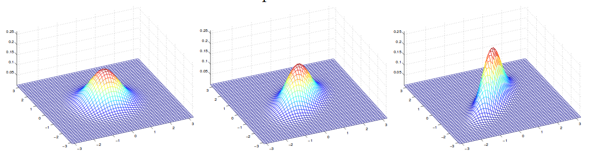
In this example, we have covariance frome left from right:

\[\Sigma = \begin{bmatrix} 1 & 0 \\ 0 & 1 \end{bmatrix}; \Sigma = \begin{bmatrix} 1 & 0.5 \\ 0.5 & 1 \end{bmatrix}; \Sigma = \begin{bmatrix} 1 & 0.8 \\ 0.8 & 1 \end{bmatrix}\]

4 GDA and logistic regression

4.1 GDA

Let’s talk about binary classification problem again. We can use multivariate Gaussian to model $p(x\lvert y)$. Put all together, we have:

\[y \sim Bernoulli(\phi)\] \[x\lvert y=0 \sim \mathcal{N}(\mu_0,\Sigma)\] \[x\lvert y=1 \sim \mathcal{N}(\mu_1,\Sigma)\]

where $\phi, \mu_0,\mu_1,\Sigma$ is the parameters that we want to find out. Note that although we have different mean for different classes, we have shared covariance between different classes.

Why is it a generative model? In short, we have a class prior on y, which is a Bernoulli. The generative process is to (1) sample a class from Bernoulli. (2) Based on the class label, we sample a x from corresponding distribution. This is generative process.

Then, the log likelihood of data is:

\[\begin{align} \ell(\phi,\mu_0,\mu_1,\Sigma) &= \log \prod_{i=1}^m p(x^{(i)}, y^{(i)};\phi,\mu_0,\mu_1,\Sigma) \\ &= \log \prod_{i=1}^m p(x^{(i)}\lvert y^{(i)};\mu_0,\mu_1,\Sigma) p(y^{(i)};\phi)\\ &= \sum\limits_{i=1}^m \log p(x^{(i)}\lvert y^{(i)};\mu_0,\mu_1,\Sigma) p(y^{(i)};\phi) \end{align}\]

In the above equation, we plug in each distribution without specifying a class. We just abstract it as k. Then, we have:

\[\begin{align} \ell(\phi,\mu_k,\Sigma) &= \sum\limits_{i=1}^m \log p(x^{(i)}\lvert y^{(i)};\mu_k,\Sigma) p(y^{(i)};\phi)\\ &= \sum\limits_{i=1}^m \bigg[-\frac{n}{2}\log 2\pi-\frac{1}{2}\log\lvert\Sigma\rvert \\ &-\frac{1}{2}(x^i-\mu_k)^T\Sigma^{-1}(x^i-\mu_k)\\ & + y^i\log\phi+(1-y^i)\log(1-\phi)\bigg]\\ \end{align}\]

Now, we need to take derivative w.r.t. each parameter and set to zero to find the argmax. Some formules might be useful for the derivation.

\(\frac{\partial x^TAx}{\partial x} = 2x^TA\) iff A is symmetric and independent of x

Proof: A is symmetric so $A=A^T$ and assume the dimension is n.

\[\begin{align} \frac{\partial x^TAx}{\partial x} &= \begin{bmatrix} \frac{\partial x^TAx}{\partial x_{1}} \\ \frac{\partial x^TAx}{\partial x_{2}} \\ \vdots \\ \frac{\partial x^TAx}{\partial x_{n}}\end{bmatrix} \\ &= \begin{bmatrix} \frac{\partial \sum\limits_{i=1}^n\sum\limits_{j=1}^n x_iA_{ij}x_j }{\partial x_{1}} \\ \frac{\partial \sum\limits_{i=1}^n\sum\limits_{j=1}^n x_iA_{ij}x_j}{\partial x_{2}} \\ \vdots \\ \frac{\partial \sum\limits_{i=1}^n\sum\limits_{j=1}^n x_iA_{ij}x_j}{\partial x_{n}} \end{bmatrix} \\ &= \begin{bmatrix} \frac{\partial \sum\limits_{i=1}^n A_{i1}x_i +\sum\limits_{j=1}^n A_{1j}x_j }{\partial x_{1}} \\ \frac{\partial \sum\limits_{i=1}^n A_{i2}x_i +\sum\limits_{j=1}^n A_{2j}x_j}{\partial x_{2}} \\ \vdots \\ \frac{\partial \sum\limits_{i=1}^n A_{in}x_i +\sum\limits_{j=1}^n A_{nj}x_j}{\partial x_{n}} \end{bmatrix} \\ &= (A + A^T)x \\ &= 2x^TA \blacksquare \end{align}\] \[\frac{\partial \log\lvert X\rvert}{\partial X} = X^{-T}\]

Jacobi’s formula:

\[\frac{\partial \lvert X\rvert}{X_{ij}} = adj^T(X)_{ij}\]

Proof:

\[\begin{align} \frac{\partial \log\lvert X\rvert}{\partial X}&=\frac{1}{\lvert X\rvert} \frac{\partial \lvert X\rvert}{\partial X} \\ &= \frac{1}{\lvert X\rvert} * adj^T (X)_{ij} \\ &= \frac{1}{\lvert X^T\rvert} * adj^T (X)_{ij} \\ &= X^{-T} \blacksquare \end{align}\] \[\frac{\partial a^TX^{-1}b}{\partial X} = -X^{-T}ab^TX^{-T}\]

Proof:

This proof is a bit complicated. You should know Kronecker delta and Frobenius inner product beforehand.

For a matrix X, we can write:

\[\frac{\partial X_{ij}}{\partial X_{kl}} = \delta_{ik}\delta{jl} = \mathcal{H}_{ijkl}\]

You can think of $\mathcal{H}$ as a identity element for the Frobenius product.

Before starting the proof, let’s prepare to find the derivative of inverse matrix. That is, $\frac{\partial X^{-1}}{\partial X}$.

\[\begin{align} I^{\prime} &= (XX^{-1})^{\prime} \\ &= X^{\prime}X^{-1} + X(X^{-1})^{\prime} \\ &= 0 \end{align}\]

So we can solve it as:

\[X(X^{-1})^{\prime} = -X^{\prime}X^{-1} \rightarrow (X^{-1})^{\prime} = X^{-1}X^{\prime}X^{-1}\]

Then, back to the original:

\[\begin{align} a^TX^{-1}b &= \sum\limits_{i,j=1}^{n,n} a_ib_j(X^{-1})_{ij} \\ &= \sum\limits_{i,j=1}^{n,n} (ab^T)_{ij}(X^{-1})_{ij} \\ &= \sum\limits_{i,j=1}^{n,n} ((ab^T)^T)_{ji}(X^{-1})_{ij} \\ &= tr(ab^T\cdot X^{-1}) \\ &= < ab^T, X^{-1}>_F \end{align}\]

where F means Frobenius inner product.

Then, plug it back:

\[\begin{align} \frac{\partial a^TX^{-1}b}{\partial X} &= \frac{\partial < ab^T, X^{-1} >_F}{\partial X} \\ &= < ab^T, \frac{\partial X^{-1}}{X} >_F \\ &= < ab^T, \frac{\partial X^{-1}}{X} >_F \\ &= < ab^T, X^{-1}X^{\prime}X^{-1} >_F \\ &= < ab^T, (X^{-T})^T X^{\prime}(X^{-T})^T >_F \\ &= < X^{-T}ab^TX^{-T},X^{\prime} >_F \\ &= < X^{-T}ab^TX^{-T},\mathcal{H} >_F \\ &= X^{-T}ab^TX^{-T} \blacksquare \end{align}\]

Now, we are good to go for finding gradient for each parameter.

For $\phi$:

\[\begin{align} \frac{\partial \ell(\phi,\mu_k,\Sigma)}{\partial \phi} &= \sum\limits_{i=1}^m (-0-0+0+\frac{y^i}{\phi}-\frac{1-y^i}{1-\phi})=0\\ &\Rightarrow \sum\limits_{i=1}^m y^i(1-\phi)-(1-y^i)\phi = 0\\ &\Rightarrow \sum\limits_{i=1}^m y^i -m\phi = 0\\ &\Rightarrow \phi = \frac{1}{m}\sum\limits_{i=1}^m \mathbb{1}\{y^{(i)}=1\} \end{align}\]

For $\mu_k$:

\[\begin{align} \frac{\partial \ell(\phi,\mu_k,\Sigma)}{\partial \mu_k} &= \sum\limits_{i=1}^m (-0-0-\frac{1}{2}2(x_k^i-\mu_k)^T\Sigma^{-1}\mathbb{1}\{y^i=k\})=0\\ &\Rightarrow \sum\limits_{i=1}^m x_k^i\mathbb{1}\{y^i=k\} - \mu_k \mathbb{1}\{y^i=k\} = 0\\ &\Rightarrow \mu_0 = \frac{\sum_{i=1}^m\mathbb{1}\{y^{(i)}=0\}x^{(i)}}{\sum_{i=1}^m\mathbb{1}\{y^{(i)}=0\}}\\ &\Rightarrow \mu_1 = \frac{\sum_{i=1}^m\mathbb{1}\{y^{(i)}=1\}x^{(i)}}{\sum_{i=1}^m\mathbb{1}\{y^{(i)}=1\}} \end{align}\]

For $\Sigma$:

\[\begin{align} \frac{\partial \ell(\phi,\mu_k,\Sigma)}{\partial \Sigma} &= \sum\limits_{i=1}^m (-\frac{1}{2}\Sigma^{-T}-\frac{1}{2} (\Sigma^{-T}(x_k^i-\mu_k)(x_k^i-\mu_k)^T\Sigma^{-T}))=0\\ &\Rightarrow \sum\limits_{i=1}^m (1-\Sigma^{-T}(x_k^i-\mu_k)(x_k^i-\mu_k)^T) = 0\\ &\Rightarrow m - \sum\limits_{i=1}^m \Sigma^{-T}(x_k^i-\mu_k)(x_k^i-\mu_k)^T = 0\\ &\Rightarrow m\Sigma = \sum\limits_{i=1}^m (x_k^i-\mu_k)(x_k^i-\mu_k)^T\\ &\Rightarrow \Sigma = \frac{1}{m}\sum\limits_{i=1}^m (x^{(i)} - \mu_{y^{(i)}})(x^{(i)} - \mu_{y^{(i)}})^T \end{align}\]

The results can be shown as:

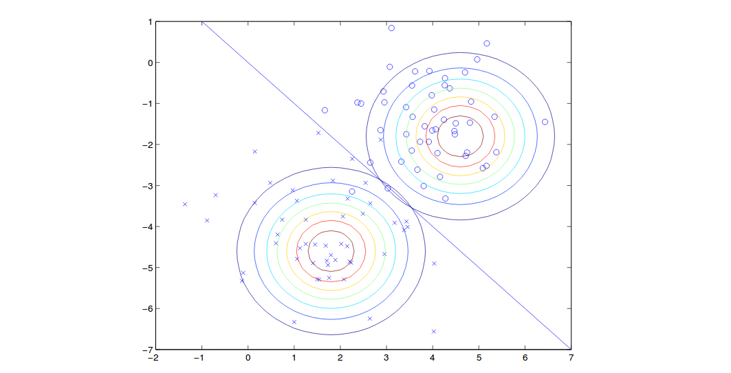
Note that we have shared covariance so the shape of two contours are the same but the means are different. On the boundary line, we have probability of 0.5 for each class.

4.2 GDA and Logistic Regression

How is GDA is related with logistic regression? We can see that if $P(x\lvert y)$ above is multivariate gaussian with shared covariance, then we can calculate $P(y\lvert x)$ and find out that it follows a logistic function. To see this, we can have:

\[p(y=1\lvert x;\phi,\mu_0,\mu_1,\Sigma) = \frac{p(x,y=1,;\phi,\mu_0,\mu_1,\Sigma)}{p(x;\phi,\mu_0,\mu_1,\Sigma)}\] \[\begin{align} &=\frac{p(y=1\lvert x;\phi)p(x\lvert \mu_1,\Sigma)}{p(y=1\lvert x;\phi)p(x\lvert \mu_1,\Sigma) + p(y=0\lvert x;\phi)p(x\lvert \mu_0,\Sigma)} \\ &= \frac{\phi\mathcal{N}(x\lvert \mu_1,\Sigma)}{\phi\mathcal{N}(x\lvert \mu_1,\Sigma) + (1- \phi)\mathcal{N}(x\lvert \mu_0,\Sigma)} \\ &= \frac{1}{1 + \frac{(1- \phi)\mathcal{N}(x\lvert \mu_0,\Sigma)}{\phi\mathcal{N}(x\lvert \mu_1,\Sigma)}} \\ \end{align}\]

Since Gaussian is member of Exponential family, we can eventually turn the ratio in the denominator to $exp(\theta^Tx)$ where $\theta$ is a function of $\phi,\mu_0,\mu_1,\Sigma$.

Similarly, if $P(x\lvert y)$ is Possion with different $\lambda$, then $P(y\lvert x)$ also follows a logistic function. It means that GDA requires a strong assumption that data of each class can be modeled with a gaussian with shared covariance. However, GDA will fit better and train faster if this assumption is correct.

On the other side, if assumption cannot be made, logistic regression is less sensitive. So you can directly use logistic regression without touching Gaussian assumption or Possion assumption.

5 Naive Bayes

In GDA, random variables are supposed to be continuous-valued. In Naive Bayes, it is for learning discrete valued random variables like text classification. Text classification is to classify text based on the words in it to a binary class. In text classification, a word vector is used for training. A word vector is like a dictionary. The length of the vector is the number of words. A word is represented by a 1 on certain position and elsewhere with 0’s in the vector.

For example, a vector of an email can be:

\[x = \begin{bmatrix} 1 \\ 1 \\ 0 \\ \vdots \\ 1 \\ \vdots \end{bmatrix}\]

where first two words might refer to “sport” and “basketball”.

However, this might not work. Say, if we have 50000 words (len(x)=50000) and try to model it as multinomial. Formally, we can model $p(x\lvert y)$ in this case where p is a multinomial. Since each word is either there or not there, which is binary case. For multinomial, we have to model all the possibility, which means the number of class is all the combinations of possible outcomes for an email. In this way, for a given class, each word can be either dependent and independent. It does not matter. We model it into Multinomial. But the dimension of parameter is $2^{50000}-1$, which is too large. Thus, to solve it, we make Naive Bayes Assumption:

Each word is conditionally independent to each other based on given class.

What it means is that if, say, an email is known in the class of sport, the appearance of word “basketball” is independent of that of word “dunk”. In this way, we can model each word indepently since we assume they are independent given a class. We can then model it as Bernoulli. We know this might not be true. That’s why we call it naive. However, based on my experience, this will give you fairly good results. Removing this assumption requires a lot of additional calculations on dependency.

Then, we have:

\[\begin{align} P(x_1,...,x_{50000}\lvert y) &=P(x_1\lvert y)P(x_2\lvert y,x_1)\\ &...P(x_{50000}\lvert y,x_1,x_2,...,x_{49999}) \\ &=\prod\limits_{i=1}^{n} P(x_i\lvert y) \end{align}\]

We apply probability law of chain rule for the first step and naive basyes assumption for the second step.

After finding the max of log joint likelihood, which is:

\[\begin{align} \mathcal{L}(\phi_y,\phi_{j\lvert y=0},\phi_{j\lvert y=1}) &= \prod\limits_{i=1}^{m} P(x^{(i)},y^{(i)}) \\ &=\prod\limits_{i=1}^{m} P(x^{(i)} \lvert y^{(i)}) P(y^{(i)}) \end{align}\]

where $\phi_{j\lvert y=1} = P(x_j = 1 \lvert y = 1)$, $\phi_{j\lvert y=0} = P(x_j = 1 \lvert y = 0)$ and $\phi_y = p(y=1)$. Those are the parameters that we want to learn. All three parameters are the parameters of Bernoulli.

We can find the derivative and solve them:

\[\begin{align} \phi_{j\lvert y=1} &= \frac{\sum_{i=1}^m \mathbb{1}\{x_j^i = 1 \text{and} y^i = 1\}}{\sum_{i=1}^m \mathbb{1}\{y^i = 1\}} \\ \phi_{j\lvert y=0} &= \frac{\sum_{i=1}^m \mathbb{1}\{x_j^i = 1 \text{and} y^i = 0\}}{\sum_{i=1}^m \mathbb{1}\{y^i = 0\}} \\ \phi_y &= \frac{\sum_{i=1}^m \mathbb{1}\{y^i = 1\}}{m} \\ \end{align}\]

Now, the number of parameters are around 100000 since 50000 parameters are learned for each given class. This is much much less than before.

To predict for a new sample, we can use Bayes Rule to calculate $P(y=1\lvert x)$ and compare which is higher.

\[p(y=1\lvert x) = \frac{p(x\lvert y=1)p(y=1)}{p(x)}\] \[=\frac{p(y=1)\prod_{j=1}^n p(x_j\lvert y=1)}{p(y=0)\prod_{j=1}^n p(x_j\lvert y=0) + p(y=1)\prod_{j=1}^n p(x_j\lvert y=1)}\]

Ext: In this case, we model $P(x_i\lvert y)$ as Bernouli since it is binary valued. That is, it can be either ‘have that word’ or ‘not have that word’. Bernouli takes class label as input and models its probability but it has to binary. To deal with non-binary valued $x_i$, we can model it as Multinomial distribution, which can be parameterized with multiple classes.

Summary: Naive Bayes is for discrete space. GDA is for continuous space. We can alsway discretize our random variable from continuous to discrete space.

6 Laplace smoothing

The above shwon example is generally good but will possibly fail where a new word which does not exist in the past training samples appear in the coming email. In such case, it would cause $\phi$ for both classes to become zero because the models never see the word before. The model will fail to make prediction.

This motivates a solution called Laplace Smoothing, which sets each parameter as:

\[\begin{align} \phi_{j\lvert y=1} &= \frac{\sum_{i=1}^m \mathbb{1}\{x_j^i = 1 \text{and} y^i = 1\}+1}{\sum_{i=1}^m \mathbb{1}\{y^i = 1\}+2} \\ \phi_{j\lvert y=0} &= \frac{\sum_{i=1}^m \mathbb{1}\{x_j^i = 1 \text{and} y^i = 0\}+1}{\sum_{i=1}^m \mathbb{1}\{y^i = 0\}+2} \\ \phi_j &= \frac{\sum_{i=1}^{m} \mathbb{1}[z^{(i)}] + 1}{m+k} \\ \end{align}\]

where k is the number of classes. In reality, the Laplace smoothing does not make too much difference since it usually has all the words but it is good to have it here.