Decision Trees

A Chinese version of this section is available. It can be found here. The Chinese version will be synced periodically with English version. If the page is not working, you can check out a back-up link here.

---

Introduction

Decision tree is one of the most popular non-linear framework used in the reality. So far, support vector machine and generalized linear are the examples of linear models. On the other hand, kernelization will result in a non-linear hypothesis function via feature mapping $\phi(x)$. Decision tree is known for its robustness to noisy and the capability of learning disjunctive expressions. In reality, decision tree has been widely used in credit risk of loan applicants.

A decision tree maps input $x\in \mathbb{R}^d$ to output y using binary rules. From top-down point of view, each node in the tree has a splitting rule. At the very bottom, each leaf node outputs an value or a class. Note, outputs can repeat. Each splitting rule can be characterized as :

\[h(x) = \mathbb{1}[x_j > t]\]

for some dimension j and $t\in \mathbb{R}$. From the leaf nodes, we can know the predictions. An example of such a decision tree can be visualized below:

Decision Trees Types

Similar to traditional prediction models, decision trees can be grouped as classification trees and regression trees. Classification trees are to classify input, while regression trees are to regress a real value in the domain as output.

Regression Trees

In this case, you can imagine that we are partitioning the space so that we can make a prediction. As an example, we have a 2 dimensional input space. We can partition each dimension individually and give a regressed value for certain region. You can visualize the idea in the left figure below.

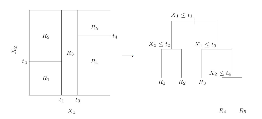
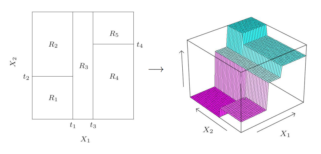
It turns out to be a tree structure such as the right one in the figure above. To predict, we assign $R_1,R_2,R_3,R_4,R_5$ to their corresponding path. In 3D space, we can see the above regression trees can lead to a stair-like partition in 3D.

Classification Trees

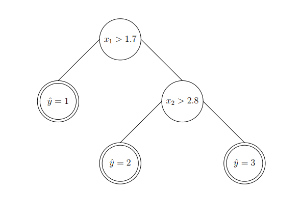
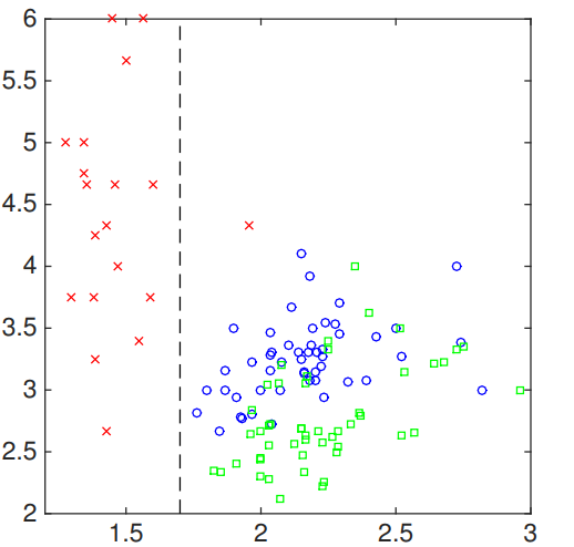
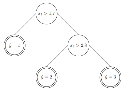
Let’s see an example of this type of decision tree. Say we have two features $x_1,x_2$ as input and 3 class labels as output. Formally, $x \in \mathbb{R}^2$ and $y \in {1,2,3}$. Figuratively, we can see:

Now, we can start from the first feature. Say we choose 1.7 as the threshold value to split. As a result,we can have:

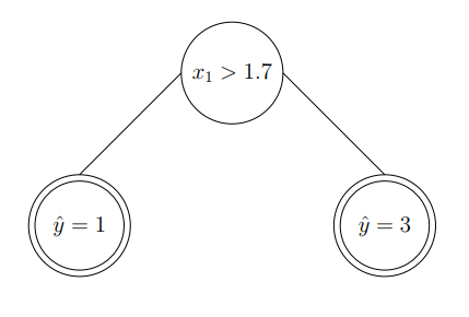
The resulted decision tree can be described as:

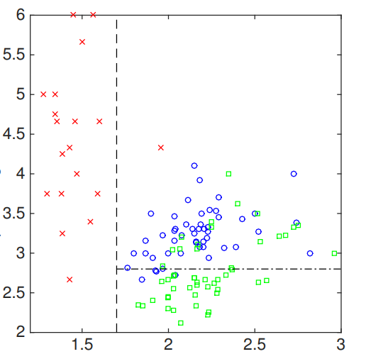
We can perform a similar action to the second feature of input. In particular, we select another threshold value along second feature space, which results in:

The resulted tree can be visualized as:

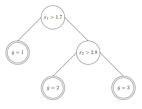
The steps above show the work flow of constructing a classification decision tree from the input space.

Learning Decision Tree

In this section, we are talking about how to learn a decision tree for both types. In general, learning trees is using a top-down greedy algorithm. In this algorithm, we start from a single node. Then, we find out the threshold value which can reduce the uncertainty the most. We keep doing this until all rules are found out.

Learning a Regression Tree

Back to the example:

In the left figure, we have five regions, two input features and four thresholds. Let’s generalize to M regions $R_1,\dots,R_M$. The prediction function can be:

\[f(x) = \sum\limits_{m=1}^M c_m \mathbb{1} \{x\in R_m \}\]

where $R_m$ is the region that x belongs to and $c_m$ is the prediction value.

The goal is to minimize:

\[\sum\limits_i (y_i - f(x_i))^2\]

Let’s look at this definition. There are two variables that need to be determined, $c_m, R_m$. The prediction is from $c_m$. So if we are given $R_m$, can we make the prediction of $c_m$ easier? The answer is yes. We can simply average all the samples in the region as $c_m$. Now, the question is how do we find out the regions?

Let’s consider to split a reigon R at the splitting value s of dimension j. The intial region is usually the entire dataset. We can define $R^{-}(j,s) = { x_i\in\mathbb{R}^d\lvert x_i(j) \leq s }$ and $R^{+}(j,s) = { x_i\in\mathbb{R}^d\lvert x_i(j) \geq s }$. Then, for each dimension j, we calculate the splitting point s that can achieve the goal the best. We should do this for each existing regirons(leaf node) so far and pick up the best region splitting based on a predefined metric.

In a word, we always select a region (leaf node), then a feature and then a threshold to form a new split.

Learning a classification decision tree.

In regression task, we use a square error to determine the quality of splitting rules. In classification task, we have more options to evaluate the quality.

Overall, there are three common measurements for classification task in growing a tree.

1, Classification error: $1 - \max_k p_k$

2, Gini Index: $1 - \sum_k p_k^2$

3, Entropy: $-\sum_k p_k \ln p_k$

where $p_k$ essentially represents the empirical portion of each class. In this case, k means the class index. For a binary classification, if we plot the value of each evaluation with respect to $p_k$, we can have:

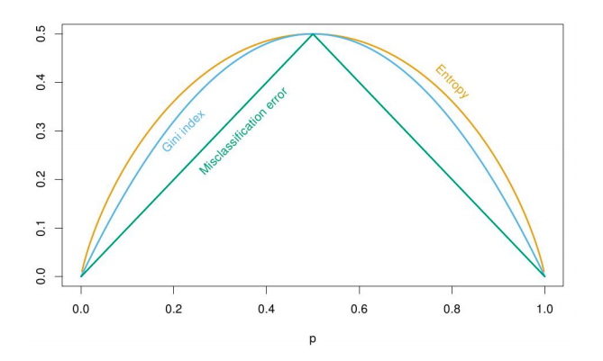
It shows that

1, all evaluations are maximized when $p_k$ is uniform on the K classes in $R_m$.

2, all evaluations are minimized when $p_k=1$ or $p_k = 0$ for some k.

In general, we always want to maximize the difference between the original loss and the cardinality-weighted loss of split regions. Formally,

\[L(R_p) = \frac{\lvert R_1\rvert L(R_1) + \lvert R_2\lvert L(R_2)}{\lvert R_1\lvert +\lvert R_2\lvert}\]

However, different loss function might have their own pros and cons. For classification error type, the problem with this type of loss is that it is insensitive to the change of splitting region. For example, if we make up a parent region $R_p$, we can depict an example like:

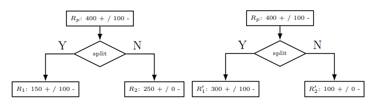
Although the splitting is different, but we can see:

\[L(R_p) = \frac{\lvert R_1\rvert L(R_1) + \lvert R_2\lvert L(R_2)}{\lvert R_1\lvert +\lvert R_2\lvert} = \frac{\lvert R_1^{\prime}\rvert L(R_1^{\prime}) + \lvert R_2^{\prime}\lvert L(R_2^{\prime})}{\lvert R_1^{\prime}\lvert +\lvert R_2^{\prime}\lvert} =100\]

We notice that different splitting results result in the same loss value if we use classification loss type. In addition, we also see that the new split regions do not reduce the original loss. Why is that? This is because classification error loss is not strictly concave. Thus, if we plot the splitting example above, we can see:

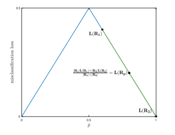
Graphically, we show the fact that the classification error loss does not help much. On the other hand, we can use entropy loss. This type of loss have a different plot.

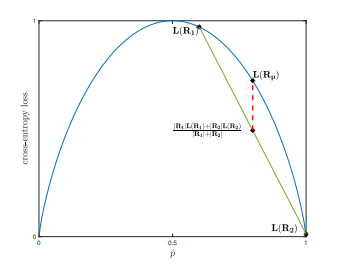
As you can see from the plot, the entropy loss will bring a reduction on the loss after we split the parent region. This is because entropy function is strictly concave.

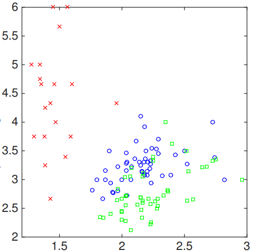
Let’s see an example of growing a classification tree using Gini index as the loss function. Let’s imagine we have a 2D space where some classified points are plotted. Such a plot can be show below.

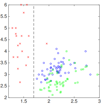
In this case, the left region $R_1$ is classified as label 1. We can see that it is classified perfectly. Thus, the measurement on this region should be perfect.

For region 2, we need to do more since Gini index is not zero. If we calculate the Gini index, we can find out:

\[G(R_2) = 1 - (\frac{1}{101})^2 - (\frac{50}{101})^2 - (\frac{50}{101})^2 = 0.5089\]

Next, we want to see how break points at different position along different axis can affect the Gini index in this region based on some evaluation function. Such a evaluation function, a.k.a. uncertainty, can be:

\[G(R_m) - (p_{r_m^-}G(R_m^-) + p_{r_m^+}G(R_m^+))\]

where $p_{R_m^+}$ is the fraction of data in $R_m$ split into $R_m^+$ and $G(R_m^+)$ is the Gina index for the new region $R_m^+$. Essentially, we want the Gini index of the new split regions to be zero. So we want to maximize the difference between the Gini index of original region and the weighted sum of Gini index on new regions. Thus, we want to plot the reduction amount on the Gini index as the function of different splitting point.

For the above example, we first look at different splitting points by sliding along with horizontal axis.

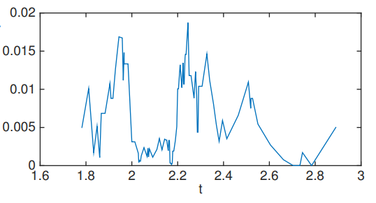
You see that there are two clear cuts on both sides because points less than approximately 1.7 belong to class 1 and no point appears after approximately 2.9. We can also experiment another setting by sliding along another axis, namely vertical axis.

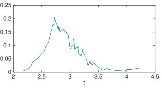
As we can see from the graph, we have the largest improvement around 2.7 as a vertical splitting point. Then, we can split our data samples as:

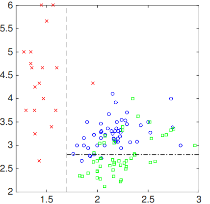
The resulted decision tree should be like:

Regularization

The question remaining is that when do we stop the growing of a tree. Naively, we can stop training when the leaf only contains one sample. However, this will lead to high variance and low bias issue, a.k.a overfitting. Some other off-the-shelf options are also available.

1, Minimum Leaf Size: we can setup a minimum number of leaf size.

2, Maximum Depth: we can also set the threshold value on the tree depth.

3, Maximum Number of Nodes: we can stop the training when the number of nodes in a tree reaches a threshold of leaf nodes.

However, even if we have these on-hand weapon to avoid overfitting, it is still hard to train a single decision tree to perform well generally. Thus, we will another useful traning technique called ensembling methods in another section.

Lack of Additive Structure

At every decision stump, one can only have one single rule based on a single feature. Features cannot be the addition from two other features. This will bring some issue for decision tree. For example, the figure below shows the case where you have to set multiple splitting points on each axis. Only one feature space is allowed at one time. That is why we always have the parallel line.

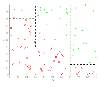
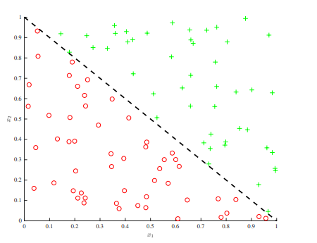
However, with additive structure, we can easily draw a linear boundary on this.