Support Vector Machine (SVM)

A Chinese version of this section is available. It can be found here. The Chinese version will be synced periodically with English version. If the page is not working, you can check out a back-up link here.

---

In this blog, I will talk about Support Vector Machine (SVM). Many people think SVM is one of the best classifier and is very easy to implment in many programming languages such as Python and Matlab. Also, I will talk about kernel idea. This allows us to apply SVM in a high dimensional space.

1 Intuition and Notation

In general, binary classification is of great interests since it is the simplest case for multi-classes classification. We have seen probabilistic models in the previous sectons such as logistic regression. On the other hand, SVM can classify points in a random dimensional space and can sovle the problem by using a deterministic algorithm.

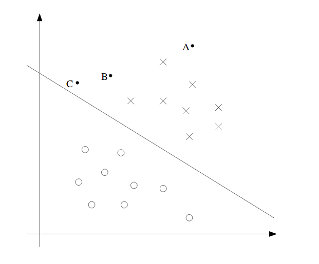
We can see an example in 2D domain above. From the figure, we have A, B and C point in the space. A is the safest point since it is far from the boundary line (hyperplane in high dimensions), while C is the most dangerous point since it is close to the hyperplane. The distance between the boundary line and the point is called margin.

We also denote $x$ as feature vector, $y$ as label and $h$ as classifier. Thus, the classifier an be shown as:

\[h_{w,b}(x) = g(w^Tx + b)\]

Note, we have w, b instead $\theta$ here. And the label only takes the value 1 and -1 instead of 0 and 1. The classifier predicts directly as 1 or -1 like perceptron algorithm without calculating the probability like what logistic algorithm does. However, some library, for example scikit-learn in Python, does provide SVM with probabilistic output. They achieve this by using a conversion function such as logistic function. Many other conversion functions are available.

2 Functional and Geometric Margins

Functional margins with respect to training example:

\[\overset{\wedge}{\gamma^{(i)}} = y^{(i)}(w^Tx^{(i)} + b)\]

We want $(w^Tx^{(i)} + b)$ to be a large positive number if label is positive or large negative number if label is negative. Thus, it means that functional margin should be positive to be correct. And the larger the margin, the more confident we are. However, this might not be meaningful when we scale w and b to 2w and 2b without changing anything else. We did not change the sign (prediction) of $(w^Tx^{(i)} + b)$ but we get a larger margin simply by scaling w and b. Thus, to make the prediction invariant to the scales of w and b, we bring a new deifnition geometric margine coming next. Furthermore, we denote the function margin for the dataset as:

\[\overset{\wedge}{\gamma} = \min_{i=1,\dots,m} \overset{\wedge}{\gamma^{(i)}}\]

where m is the number of training samples.

Geometric Margins: In geometric margin, we need to normalize w and b with respect to the norm of w since we think the magnitude of w and b should not affect the scale of the margin. A figure for geometric margin can be shown:

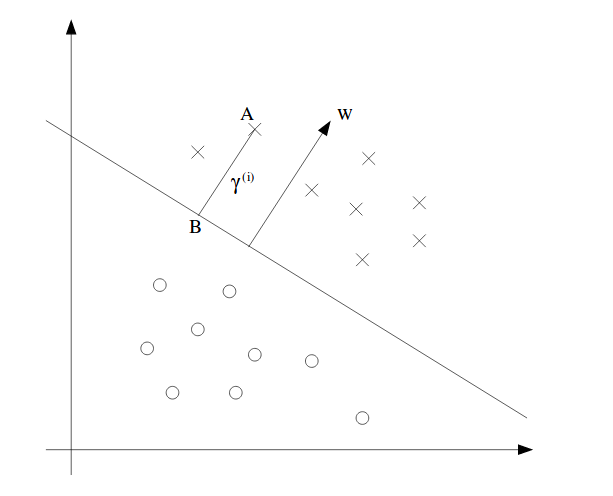
It shows a vector w also called support vector which is perpendicular to the boundary line, which is always true. To prove this, let’s take any two points on the line, $x_i,x_j,i\neq j$. Since two points are on the line, by definition, we have:

\[w^T x_i + b = w^T x_j + b = 0\]

Then, we can say:

\[w^T(x_i-x_j) = 0\]

$x_i-x_j$ is the vector along the line. We know that dot product is always zero and it is always perpendicular between the two vectors.

Similarily, to find the margin of point A, denoted $\gamma^{(i)}$ which is a scalar, we take point B as the projected point of A on the line. By definition, $x^{(i)} - \gamma^{(i)} w/\lvert\lvert w \rvert\rvert$. The point is on boundary, meaning that

\[w^T(x^{(i)} - \gamma^{(i)} \frac{w}{\lvert\lvert w \rvert\rvert}) + b = 0\]

Solve:

\[\gamma^{(i)} = (\frac{w}{\lvert\lvert w \rvert\rvert})^T x^{(i)} + b/\lvert\lvert w \rvert\rvert\]

This is for the positive case. So the margin is positive. For negative samples, we get a negative number. To unify this, we multiply the label to the derived margin above. Thus, geometric margin with respect to a training sample is defined as:

\[\gamma^{(i)} = y^{(i)}((\frac{w}{\lvert\lvert w \rvert\rvert})^T x^{(i)} + b/\lvert\lvert w \rvert\rvert)\]

If $\lvert\lvert w \rvert\rvert = 1$, the functional margin is equal to geometric margin. The geometric margin is invariant to rescaling of the parameteres. It means that if we scale w and b by 2, we will still have the same geometric margin (not functional margin). Keep in mind that you have to scale both parameters by same scalar. The key idea is that we can get whatever functional margin we want but still have the same geometric margin.

Similarily, the geometric margin for all samples is:

\[\gamma = \min_{i=1,\dots,m}\gamma^{(i)}\]

3 Optimal Margin Classifier (OMC)

Most importantly, I will keep it short: the goal is to maximize the geometric margin. The larger, the better.

For now, we assume that data is linearly separable. The optimization problem can be defined as :

\[\begin{align} \max_{\gamma,w,b} & \gamma \\ \text{s.t. } & y^{(i)}(w^Tx^{(i)} + b) \geq \gamma, i = 1,\dots,m \\ & \lvert\lvert w \rvert\rvert = 1 \end{align}\]

The first constraint is to ensure that every training sample has a valid geometric margin. The second constraint is to ensure that geometric margin is equal to functional margin. We have to have the second constraint since $y^{(i)}(w^Tx^{(i)} + b)$ is functional margin. By having the second constraint, we make functional margin equal to geometric margin. The nasty point is $\lvert\lvert w \rvert\rvert = 1$ constraint, which makes it non-convex. If it is convex, we can get the derivative and set to zero. This is another topic.

To facilitate this, we can then transform it to:

\[\begin{align} \max_{\overset{\wedge}{\gamma},w,b} & \frac{\overset{\wedge}{\gamma}}{\lvert\lvert w \rvert\rvert} \\ \text{s.t. } & y^{(i)}(w^Tx^{(i)} + b) \geq \overset{\wedge}{\gamma}, i = 1,\dots,m \end{align}\]

Basically, we express geometric margin using function margin. Instead of geometric margin, we subject to a functional margin, which is originally expected. By doing this, we eliminate $\lvert\lvert w \rvert\rvert = 1$. However, it is still bad.

Recall that by scaling w and b, we do not change anything. We use this fact to force the functional margin $\overset{\wedge}{\gamma} = 1$ but do not change the geometric margin. And then, the max problem can be expressed as a min problem now. That is,

\[\begin{align} \min_{\gamma,w,b} & \frac{1}{2} \lvert\lvert w \rvert\rvert^2 \\ \text{s.t. } & y^{(i)}(w^Tx^{(i)} + b) \geq 1, i = 1,\dots,m \end{align}\]

Again, the reason we have $\frac{1}{2}$ is just for math convenience. It does not hurt anything. The problem can be solved by using quadratic programming software. We can still go further to simplify this but it requires the knowledge of Lagrange Duality

4 Lagrange Duality

Let’s take a side step on how to solve general constrained optimizing problem. In general, we usually use Lagrange Duality to solve this type of question.

Consider a problem such as :

\[\begin{align} \min_w & f(w) \\ \text{s.t. } & h_i(w) = 0,i = 1,\dots,l \end{align}\]

Now, we can define Lagrangian to be:

\[\mathcal{L}(w,\beta) = f(w) + \sum\limits_{i=1}^l \beta_i h_i(w)\]

where $\beta_i$ is called Lagrange multiplier. Now, we can use partial derivative to set to zero and find out each $w_i$ and each $\beta_i$.

The above only has equality constraints. We can generalize to both inequality and equality constraints. So we can define primal problem to be:

\[\begin{align} \min_w & f(w) \\ \text{s.t. } & g_i(w) \leq 0,i = 1,\dots,k \\ & h_i(w) = 0,i = 1,\dots,l \end{align}\]

We define generalized Lagrangian as:

\[\mathcal{L} = f(w) + \sum\limits_{i=1}^k \alpha_i g_i(w) + \sum\limits_{i=1}^l \beta_i h_i(w)\]

where all $\alpha$ and $\beta$ are Lagrangian multiplier.

Let’s define a quantity for primal problem as:

\[\theta_{\mathcal{P}}(w) = \max_{\alpha,\beta:\alpha_i\geq 0} \mathcal{L}(w,\alpha,\beta)\]

In this quantity, we need $\alpha_i$ to be larger than zero. If $\alpha_i < 0$, the max of the above quantity is just $\infty$ since $g_i(w) \leq 0$. Also if some constraints are violated, then $\theta_{\mathcal{P}}(w) = \infty$ as a result.

If everything is satisfied, we have:

\[\theta_{\mathcal{P}}(w) = \begin{cases} f(w) \text{, if w satisfy primal constraints} \\ \infty \text{, otherwise} \\ \end{cases}\]

To mathch with our primal problem, we define the min problem as:

\[\min_w \theta_{\mathcal{P}}(w) = \min_w \max_{\alpha,\beta:\alpha_i\geq 0} \mathcal{L}(w,\alpha,\beta)\]

This is the same as the primal problem if all constrain are satisfied. We define the value of primal problem to be: $p^{\ast} = \min_w \theta_{\mathcal{P}(w)}$.

Then, from different perspectives, we can define:

\[\theta_{\mathcal{D}}(\alpha,\beta) = \min_w \mathcal{L}(w,\alpha,\beta)\]

to be part of the dual problem. To again match with the primal problem, we define the dual optimization problem to be:

\[\max_{\beta,\alpha:\alpha_i\geq 0} \theta_{\mathcal{D}}(\alpha,\beta) = \max_{\alpha,\beta:\alpha_i\geq 0} \min_w \mathcal{L}(w,\alpha,\beta)\]

Similarily, the value of dual problem is $d^{\ast} = \max_{\alpha,\beta:\alpha_i\geq 0} \theta_{\mathcal{D}}(\alpha,\beta)$

The primal and dual problem is related by:

\[d^{\ast} = \max_{\alpha,\beta:\alpha_i\geq 0} \theta_{\mathcal{D}}(\alpha,\beta) \leq p^{\ast} = \min_w \theta_{\mathcal{P}(w)}\]

This is always true. To see this, let’s first define a function $f(x,y): X \times Y \mapsto \mathbb{R}$. Then, we can define:

\[g(x) := \min_{y} f(x,y)\]

That is for every x of funciton g, we choose such a y value that f(x,y) is minimum. Then, we can say:

\[g(x) \leq f(x,y) \forall x\forall y\]

We can add a max operator on both sides so as to eliminate variable x. In particular,

\[\max_{x} g(x) \leq \max_{x} f(x,y) \forall y\]

This is equivalently saying:

\[\max_{x} \min_{y} f(x,y) \leq \min_{y} \max_{x} f(x,y)\]

This concludes the proof.

Back to the topic: The key is that under certain condition, they are equal. If they are equal, we can focus on dual problem instead of primal problem. The question is when they are equal.

We assume that f and g are all convex and h are affine(When f has a Hessian, it is convex iff Hessian is positive semi-definite. All affine are convex. Affine means linear.) and g are all less than 0 for some w. Wtih these assumptions, there must exist $w^{\ast}$ for primal solution and $\alpha^{\ast},\beta^{\ast}$ for dual solution and $p^{\ast} = d^{\ast}$. And $w^{\ast}$,$\alpha^{\ast}$ and $\beta^{\ast}$ satisfy Karush-Kuhn-Tucker (KKT) conditions, which says:

\[\frac{\partial}{\partial w_i}\mathcal{L}(w^{\ast},\alpha^{\ast},\beta_{\ast}) = 0. i = 1,\dots,n\] \[\frac{\partial}{\partial \beta_i}\mathcal{L}(w^{\ast},\alpha^{\ast},\beta_{\ast}) = 0. i = 1,\dots,l\] \[\alpha_i^{\ast}g_i(w^{\ast}) = 0,i = 1,\dots,k\] \[g_i(w^{\ast}) \leq 0,i = 1,\dots,k\] \[\alpha_i^{\ast} \geq 0,i = 1,\dots,k\]

Third euqaiton is called KKT dual complementarity condition. It means if $\alpha_i^{\ast} > 0$, then $g_i(w^{\ast}) = 0$. When we find out the state where primal problem is equal to dual problem, every conditions and assumtions above should be met.

5 OMC with Lagrange Duality

Let’s revisit the primal problem in SVM:

\[\begin{align} \min_{\gamma,w,b} & \frac{1}{2} \lvert\lvert w \rvert\rvert^2 \\ \text{s.t. } & y^{(i)}(w^Tx^{(i)} + b) \geq 1, i = 1,\dots,m \end{align}\]

we can re-arrange the constraint to be:

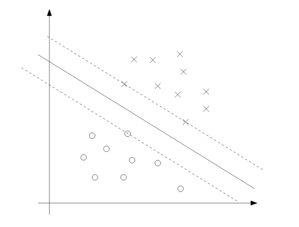
\[g_i(w) = -y^{(i)}(w^Tx^{(i)} + b) + 1 \leq 0\]

where i spans all training samples. From KKT dual complementarity condition, we have $\alpha_i > 0$ only when the functional margin is 1 where $g_i(w) = 0$.

We can visualize this in the picture below. The three points on the dash line are the ones with the smallest margin which is 1. Thus, those points are the ones with positve $\alpha_i$ and are called support vector.

The Lagranian with only inequality constraint is:

\[\mathcal{L}(w,b,\alpha) = \frac{1}{2}\lvert \lvert w\rvert \rvert^2 - \sum\limits_{i=1}^m \alpha_i [y^{(i)}(w^Tx^{(i)} + b) - 1] \tag{1}\]

To find the dual form of this problem, we first find the min of loss function with respect to w and b for a fixed $\alpha$. To do that, we have:

For w:

\[\triangledown_{w}\mathcal{L}(w,b,\alpha) = w - \sum\limits_{i=1}^m \alpha_i y^{(i)}x^{(i)} = 0\tag{2}\]

This means:

\[w = \sum\limits_{i=1}^m \alpha_i y^{(i)}x^{(i)}\tag{3}\]

For b:

\[\frac{\partial}{\partial b}\mathcal{L}(w,b,\alpha) = \sum\limits_{i=1}^m \alpha_i y^{(i)} = 0 \tag{4}\]

A useful formaul is:

\[\begin{align} \lvert\lvert\sum\limits_{i=1}^m \alpha_i y^{(i)}x^{(i)}\rvert\rvert^2 &= (\sum\limits_{i=1}^m \alpha_i y^{(i)}x^{(i)})^T(\sum\limits_{i=1}^m \alpha_i y^{(i)}x^{(i)}) \\ &= \sum\limits_{i,j}^m y^{(i)}y^{(j)}\alpha_i\alpha_j (x^{(i)})^Tx^{(j)} \end{align}\]

We take equation (3) back to equation (1) we have:

\[\begin{align} \mathcal{L}(w,b,\alpha) &= \frac{1}{2}\sum\limits_{i,j}^m y^{(i)}y^{(j)}\alpha_i\alpha_j (x^{(i)})^Tx^{(j)} \\ & - \sum\limits_{i=1}^m \alpha_i [y^{(i)}((\sum\limits_{j=1}^m \alpha_j y^{(j)}x^{(j)})^Tx^{(i)} + b) - 1] \\ &= \frac{1}{2}\sum\limits_{i,j}^m y^{(i)}y^{(j)}\alpha_i\alpha_j (x^{(i)})^Tx^{(j)} - \sum\limits_{i,j}^m y^{(i)}y^{(j)}\alpha_i\alpha_j (x^{(i)})^Tx^{(j)} \\ & - b\sum\limits_{i=1}^m\alpha_i y^{(i)} + \sum\limits_{i=1}^m \alpha_i \\ &= \sum\limits_{i=1}^m \alpha_i - \frac{1}{2}\sum\limits_{i,j}^m y^{(i)}y^{(j)}\alpha_i\alpha_j (x^{(i)})^Tx^{(j)} \end{align}\]

Note that $\alpha_i \geq 0$ and constraint (4). Thus, we have the dual problem as:

\[\begin{align} \max_{\alpha} W(\alpha) &= \sum\limits_{i=1}^m \alpha_i - \frac{1}{2}\sum\limits_{i,j}^m y^{(i)}y^{(j)}\alpha_i\alpha_j <x^{(i)},x^{(j)}> \\ \text{s.t. } & \alpha_i \geq 0, i = 1,\dots,m \\ & \sum\limits_{i=1}^m \alpha_i y^{(i)} = 0 \end{align}\]

which satisfies KKT condition (You can check it). It means we found out the dual problem to solve instead of primal problem. If we can find $\alpha$ from this dual problem, we can use equation (3) to find $w^{\ast}$. With optimal $w^{\ast}$, we can find $b^{\ast}$:

\[b^{\ast} = -\frac{\max_{i:y^{(i)}=-1}w^{\ast T}x^{(i)} + \min_{i:y^{(i)}=1}w^{\ast T}x^{(i)}}{2}\]

This is easy to verify. Basically, we just take the two points from positive class and negative class that have the same distance to the hyperplane. That is, they are support vectors. The margin they are are euqal and this property can be used to solve for $b^{\ast}$. The optimal w and b will make the geometric margin of cloest negative and positive sample to be equal.

The equation (3) says that the optimal w is based on the optimal $\alpha$. To make prediction, then we have:

\[w^Tx + b = (\sum\limits_{i=1}^m \alpha_i y^{(i)} x^{(i)})^Tx + b = \sum\limits_{i=1}^m \alpha_i y^{(i)} <x^{(i)},x> + b\]

If it is bigger than zero, we predict one.If it is less than zero, we predict negative one. We also know that $\alpha$ will be all zeros except for the support vectors because of the constraints. That means we only cares about the inner product between x and support vector. This makes the prediction faster and brings the Kernel funciton into the sight. Keep in mind that so far everything is low dimensional. How about high dimensions and infinite dimension space?

6 Kernels

In the example of living area of house, we can use the feature $x,x^2,x^3$ to get cubic function where x can be the size of house. X is called input attribute and $x,x^2,x^3$ is called features. We dentoe a feature mapping function $\phi (x)$ that maps from attribute to features.

Thus, we might want to learn in the new feature space $\phi (x)$. In last section,we only need to calculate inner product $<x,z>$ and now we can replace it with $<\phi(x),\phi(z)>$.

Formally, given a mapping, we denote Kernel to be:

\[K(x,z) = \phi(x)^T\phi(z)\]

We can use Kernel instead of mapping itself. The reason can be found in the original notes. I am not talking details here. In short, the reason is that Kernel is less expensive computationally and can be used for high/infinite dimensional mapping. So we can learn in high dimensuional space without calculating mapping function $\phi$.

An example of how effective it is can be shown in the notes. It should be noted that calculating mapping is exponential time complexity whereas Kernel is linear time.

In another way, Kernel is a measurement of how close or how far it is between two samples: x and z. It indicates the concepts of similarity. One of the popular Kernel is called Gaussian Kernel defined as:

\[K(x,z) = \exp(-\frac{\lvert\lvert x-z \rvert\rvert^2}{2\sigma^2})\]

We can use this as learning SVM and it corresponds to infinite dimensional feature mapping $\phi$. It means that the mapping funciton $\phi$ is infinite. It also shows that it is impossible to calculate infinite dimensional mapping but we can use Kernel instead.

Next, we are interested in telling if a given Kernel is valid or not.

We define Kernel Matrix as $K_{ij} = K(x^{(i)},x^{(j)})$ for m points(i.e. K is m-by-m). Now, if K is valid, it means:

(1)Symmetric: $K_{ij} = K(x^{(i)},x^{(j)}) = \phi(x^{(i)})^T\phi(x^{(j)}) = \phi(x^{(j)})^T\phi(x^{(i)}) = K_{ji}$

(2)Positive semi-definite: $z^TKz \geq 0$ proof is easy, will provide if necessary.

Mercer Theorem: Let $K:\mathbb{R}^n \times \mathbb{R}^n \mapsto \mathbb{R}$ be given. Then for a Kernel to be valid, it is necessary and sufficient that for any ${x^{(1)},\dots,x^{(m)}}$, the corresponding kernel matrix is symmetric and postive semi-definite.

Since Kernel method does allow us to project low dimensional vector to a higher dimensionality, this explains why dual problem is preferred than primal problem in general.

Kernel method is not only used in SVM but also everywhere inner product is used. So we can replace the inner product with Kernel so that we can work in a higher dimensional space.

7 Regularization and Non-separable Case

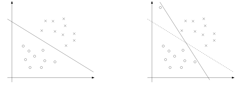
Although mapping x to higher dimensional space increases the chance to be separable, it might not always be the case. An outlier could also be the cause that we actually don’t want to include. An example of such a case can be shown below.

To make the algorithm work for non-linear case as well, we add regularization to it:

\[\begin{align} \min_{\gamma,w,b} & \frac{1}{2}\lvert\lvert w\rvert\rvert^2 + C\sum\limits_{i=1}^m \xi_i \\ \text{s.t. } & y^{(i)}(w^Tx^{(i)} + b) \geq 1-\xi_i,i=1,\dots,m \\ & \xi_i \geq 0,i=1,\dots,m \end{align}\]

It will pay the cost for the functional margin that is less than one. C will ensure that most examples have functional margin at least 1. It says that:

(1) We want w to be small so that margin will be large.

(2) We want most samples to have functional margin that is larger than 1.

The Lagrangian is :

\[\begin{align} \mathcal{L}(w,b,\xi,\alpha,r) &= \frac{1}{2}w^Tw + C\sum\limits_{i=1}^{m}\xi_i \\ & - \sum\limits_{i=1}^m \alpha_i[y^{(i)}(x^{(i)T}w + b) - 1 + \xi_i] - \sum\limits_{i=1}^{m}r_i\xi_i \end{align}\]

where $\alpha$ and r are Lagrangian multipliers which must be non-negative since constraints here are inequality. Now, we need to do the same thing to find out the dual form of the problem. I ignore the procedure here. After setting the derivatives with respect to w and b to zero, plugging back will produce the dual problem as:

\[\max_{\alpha} W(\alpha) = \sum\limits_{i=1}^{m}\alpha_i - \frac{1}{2}\sum\limits_{i,j=1}^{m}y^{(i)}y^{(j)}\alpha_i\alpha_j<x^{(i)},x^{(j)}>\] \[\text{s.t. }0\leq \alpha_i \leq C,i=1,\dots,m\] \[\sum\limits_{i=1}^{m}\alpha_i y^{(i)} = 0\]

Notice that we have an interval for $\alpha$. This is becuase it has $\sum\limits_{i=1}^{m}(C-\alpha_i-r_i)\xi_i$. We take derivative with respect to $\xi$ and set to zero and we can eliminate $\xi$ and get the interval. In this case, $r_i$ is always non-negative and $\alpha_i=C$ when $r_i = 0$.

Also notice that the optimal b is not the same anymore because the margin for both cloest points have changed. In next section, we will find the algrotihm to figure out the solution.

8 The SMO Algorithm

The SMO(sequential minimal optimization) algorithm by John Platt is to solve the dual problem in SVM.

8.1 Coordinate Ascent

In general, the optimization problem

\[\max_{\alpha}W(\alpha_1,\alpha_2,\dots,\alpha_m)\]

can be solved by gradient ascent and Newton’s method. In addition, we can also use coordinate ascent:

for loop until convergence:
  for i in range(1,m):
    alpha(i) = argmin of alpha(i) W(all alpha)

Basically, we fix all the $\alpha$ except for $\alpha_i$ and then move to next $\alpha$ for updating. The assumption is that calculating gradient to $\alpha$ is efficient. An example can be shown below.

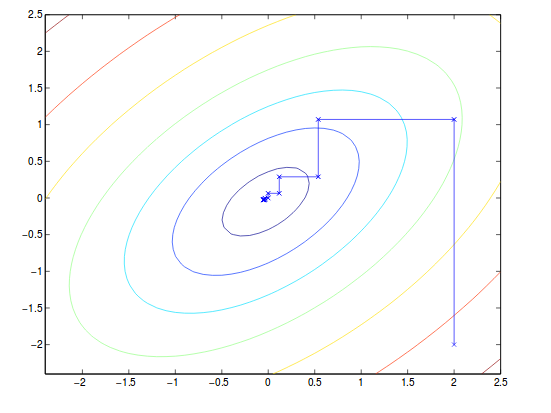
Note that the path of the convergence is always parallel to axis because it is updated one variable at a time.

8.2 SMO

We cannot do the same thing in dual problem in SVM because varying only one variable might violate the constraint:

\[\alpha_1 y^{(1)} = -\sum\limits_{i=2}^m \alpha_i y^{(i)}\]

which says once we determine the rest of $\alpha$, we cannot vary the left $\alpha$ anymore. Thus, we have to vary two $\alpha$ at one time and update them. For exmaple, we can have:

\[\alpha_1 y^{(1)} + \alpha_2 y^{(2)} = -\sum\limits_{i=3}^m \alpha_i y^{(i)}\]

We make right side to be constant:

\[\alpha_1 y^{(1)} + \alpha_2 y^{(2)} = \zeta\]

which can be pictorially shown as:

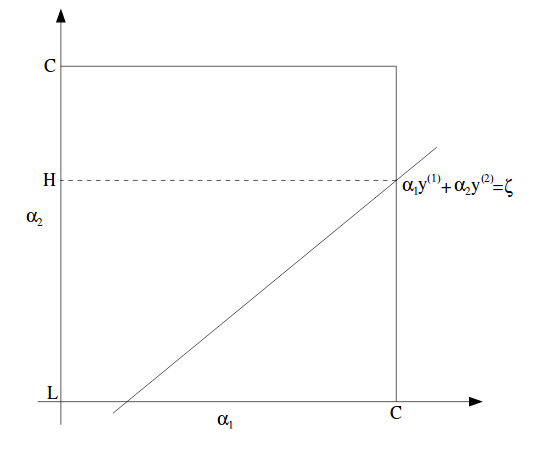
In this figure, L and H are the lowest possible and highest possible value for $\alpha_2$, while $\alpha_1$ is between 0 and C.

Note that although it is a square where $\alpha$ can lie but with a straight line, we might have a lower bound and upper bound on them.

We can rewrite the above equation:

\[\alpha_1 = (\zeta - \alpha_2 y^{(2)})y^{(1)}\]

Then, W will be :

\[W(\alpha_1,\dots,\alpha_m) = W((\zeta-\alpha_2 y^{(2)})y^{(1)},\alpha_2,\dots,\alpha_m)\]

We treat all other $\alpha$ as constants.Thus, after plugging in, W will become quadratic, which can be written as $a\alpha_2^2 + b\alpha_2 + c$ for some a, b and c.

Last, we define $\alpha_2^{new, unclipped}$ as the current solution to update $\alpha_2$. Thus, with applying constraints, only for this single variable, we can write:

\[\alpha_2^{new} = \begin{cases} H \text{, if }\alpha_2^{new, unclipped}>H \\ \alpha_2^{new, unclipped} \text{, if } L\leq \alpha_2^{new, unclipped} \leq H \\ L \text{, if } \alpha_2^{new, unclipped} < L \\ \end{cases}\]