Learning Theory

1 Bias-Varaince tradeoff

This has already been discussed in last section. In additon, we should emphasize that:

1) A simple model with few parameters should have low variance on its prediction but will produce a high bias in general.

2) A complex model with too many parameters to train usually have a high variance although it can predict well(low bias).

There is a tradeoff in between.

2 Preliminaries

The key idea is to formalize the analysis on a machine learning algorithm. For example, is there a bound on generalization error? Is there condition on that limit? How can we select a model over others? This is what learning theory talks about.

We start off by introducing two lemmas:

Lemma (The Union Bound) Let $A_1,A_2,\dots,A_k$ be k different events, which might not be independent. Then:

\[P(A_1\cup\dots\cup A_k)\leq P(A_1)+ \dots + P(A_k)\]

This, Union Bound, is a common used axiom in learning theory. The proof can be easily found online.

Lemma (Hoeffding Inequality) Let $Z_1,Z_2,\dots,Z_m$ be m iid random variables drawn from Bernoulli($\phi$) distribution. That is: $P(Z_i = 1) = \phi, P(Z_i = 0) = 1 - \phi$. Let $\hat{\phi} = \frac{1}{m}\sum_{i=1}^m Z_i$ be the mean of random variable and let $\gamma > 0$ be fixed. Then:

\[P(\lvert \phi - \hat{\phi}\rvert >\gamma)\leq 2\exp(-2\gamma^2m)\]

This is a.k.a Chernoff bound. Think about what it says. If we take the mean of r.v. as the estimation of future input, then the probability of the discrepance between truth and the estimation larger than a threshold is less than a value related with the number of training samples and the threshold as well. This is frequently used in learning theory.

This lemma can be generalized to multi-class classification as well but we just focus on binary case for now. Assume that we have a training set S with m pairs of sample. Each $(x^{(i)},y^{(i)})$ pair are drawn iid from some distribution $\mathcal{D}$. For a hypothesis h, we define the training error or empirical risk to be:

\[\hat{\varepsilon}(h) = \frac{1}{m}\sum\limits_{i=1}^m \mathbb{1}\{h(x^{(i)}\neq y^{(i)}\}\]

We also define the generalization error to be:

\[\varepsilon(h) = P_{(x,y)\thicksim \mathcal{D}}(h(x)\neq y)\]

This quantity shows how much probability of misclassification will be if we sample one pair from the distribution $\mathcal{D}$. The above concepts are often related to probably approximately correct(PAC) problem, which has two most important assumption:(1)training and testing samples are from the same distribution. (2) each pair of sample is iid. In short, the empirical risk is the error resulted from training data that we are currently holding, whereas the generalization error is the error resulted from samples drawn from the same distribution as training dataset.

Think about linear classification again. We can let $h_{\theta}(x) = \mathbb{1}\{\theta^Tx\geq 0\}$ to be our hypothesis. The goal is to find $\theta$ which can minimize the training error. Formally,

\[\hat{\theta} = \arg\min_{\theta}\hat{\varepsilon}(h_{\theta})\]

This is called empirical risk minimization(ERM). The output hypothesis is $h_{\hat{\theta}}$. The ERM is the core idea of learning algorithm. Logisitic regression problem can also be analog to this algorithm.

In learning theory, we do not want to restrict the hypothesis to a linear classifier or so. We want it to point out a general hypothesis form. Thus, we define the hypothesis class $\mathcal{H}$ to be the set of all classifiers in the case. In this set, all valid classifiers are considered against to a evaluation scheme. Concequently, ERM can be treated as the minimization over the class of functions $\mathcal{H}$. Formally:

\[\hat{h} = \arg\min_{h\in\mathcal{H}}\hat(\varepsilon)(h)\]

3 The Case of Finite $\mathcal{H}$

To begin with, we first consider the case where the number of hypothesis classes is finite, dentoed $\mathcal{H} = {h_1,h_2.\dots,h_k}$ for k hypotheses. Each hopythosis is just a mapping function which takes $\mathcal{x}$ as input and map to either 1 or 0 and ERM algorithm is just to select the hypothesis which produces minimum training error, namely $\hat{h}$.

So now the question is what we can say about generalization error on $\hat{h}$. For exmaple, can we give a bound on the error? If so, it implies that in any circumstances, the error rate would not exceed the bound we derived. To do so, we need (1) to show $\hat{\varepsilon}(h)$ is a good estimate of $\hat{\varepsilon}(h)$ for all h. (2) to show that this implies an upper-bound on the generalization error of $\hat{h}$.

We pick $h_i$ from $\mathcal{H}$ and denote $Z=\mathbb{1}\{h_i(x) \neq y\}$ where $(x,y)\thicksim\mathcal{D}$. Basically, Z indicates if $h_i$ misclassifies it. And we also denote $Z_j = \mathbb{1}\{h_i(x^{(i)}) \neq y^{(i)}\}$. Note that since all samples are drawn from D, thus $Z$ and $Z_i$ have the same distribution.

We should notice that $\mathbb{E}[Z] = \mathbb{E}[\mathbb{1}\{h_i(x) \neq y\}] = P_{(x,y)\thicksim \mathcal{D}}(h(x)\neq y) = \varepsilon(h)$ which also applies for $Z_j$. It represents the probability of misclassification on a random sample. Moreover, the training error can be written:

\[\hat{\varepsilon}(h_i) = \frac{1}{m}\sum\limits_{j=1}^m Z_j\]

We can see that $\hat{\varepsilon}(h_i)$ is exactly the mean of m random variables $Z_j$ drawn iid from Bernoulli distribution with mean $\varepsilon(h_i)$. We can apply Hoeffding inequality as:

\[P(\lvert\varepsilon(h_i)-\hat{\varepsilon}(h_i)\rvert > \gamma)\leq 2\exp(-2\gamma^2m)\]

This means that for a particular $h_i$ with high probablity the empirical error will be close to generalization error. which is nice. The more valueable point is to prove this is true for all $h\in\mathcal{H}$.

To do this, we denote $A_i$ be the event that $\lvert\varepsilon(h_i) - \hat{\varepsilon}(h_i)\rvert>\gamma$. In the above, we have proved that for a particular $A_i$, it is true that $P(A_i)\leq 2\exp(-1\gamma^2m)$. With union bound, we have:

\[\begin{align} P(\exists h_i\in \mathcal{H}.\lvert \varepsilon(h_i)-\hat{\varepsilon}(h_i)>\gamma) &= P(A_1\cup A_2\cup\dots\cup A_k)\\ &\leq \sum\limits_{i=1}^k P(A_i) \\ &\leq \sum\limits_{i=1}^k 2\exp(-2\gamma^2m)\\ &= 2k\exp(-2\gamma^2m) \end{align}\]

If we substract 1 from both sides, we have:

\[\begin{align} P(\neg\exists h_i\in \mathcal{H}.\lvert \varepsilon(h_i)-\hat{\varepsilon}(h_i)>\gamma) &= P(\forall h_i\in \mathcal{H}.\lvert \varepsilon(h_i)-\hat{\varepsilon}(h_i)\leq\gamma)\\ &\geq 1-2k\exp(-2\gamma^2m) \end{align}\]

This simply says that with probability at least $1-2k\exp(-2\gamma^2m)$, we have generalization error to be within the bound of empirical error for all $h\in \mathcal{H}$. It is called uniform convergence result.

In this case, we are really interested in 3 quantities: $m,\gamma$ and probability of error, denoted as $\delta$. The reason that we are interested in these three variables is because they are correlated in some way. For example, given $\gamma$ and some $\delta>0$, we can find m by solving $\delta = 2k\exp(-2\gamma^2m)$:

\[m\geq\frac{1}{2\gamma^2}\log\frac{2k}{\delta}\]

This quantity says about how many training samples are required to make the bound valid, which is only logarithmic in k. It is also called sample complexity.

Similarly, given m and $\delta$, we can solve for $\gamma$ and we will get:

\[\lvert\hat{\varepsilon}(h) - \varepsilon(h)\rvert\leq\sqrt{\frac{1}{2m}\log\frac{2k}{\delta}}\]

Assume that the uniform convergence holds for all hypotheses, can we also bound the generalization error on $\hat{h}=\arg\min_{h\in\mathcal{H}}\hat{\varepsilon(h)}$?

Define $h^{\ast} = \arg\min_{h\in\mathcal{h}}\varepsilon(h)$ to be the best possible hypothesis. We are trying to compare the hypothesis which achieves the best in training data and that which does the best in generalization error theorectically. We have:

\[\begin{align} \varepsilon(\hat{h}) &\leq \hat{\varepsilon}(\hat{h}) + \gamma\\ &\leq \hat{\varepsilon}(h^{\ast}) + \gamma\\ &\leq \varepsilon(h^{\ast}) + 2\gamma \end{align}\]

The first line is by definition $\lvert \varepsilon(\hat{h}) -\hat{\varepsilon}(\hat{h})\rvert \leq \gamma$, which is similar for the third line as well. From this proof, we have shown that if uniform convergence occurs, the generalization error of empirically selected h is at most $2\gamma$ worse than per generalization-error selected hypothesis in $\mathcal{H}$.

Theorem Let $\lvert \mathcal{H} \rvert = k$,and let $m,\delta$ be fixed. Then with probability at least $1-\delta$, we have:

\[\varepsilon(\hat{h})\leq \bigg(\min_{h\in\mathcal{H}}\varepsilon(h)\bigg)+2\sqrt{\frac{1}{2m}\log\frac{2k}{\delta}}\]

This is related to bias-variance tradeoff as well. Assum that we have a larger hypothesis class $\mathcal{H}^{\prime}$ where $\mathcal{H} \supseteq \mathcal{H}^{\prime}$. If we learn on the new hypothesis class, we have a bigger k. Thus, the second term above will be larger. That is, the variance will be larger. However, the the first term is smaller. That is the bias will go down.

Corollary Let $\lvert\mathcal{H}\rvert=k$ and given $\delta,\gamma$, then for $\varepsilon(\hat{h})\leq\min_{h\in\mathcal{H}}\varepsilon(h) + 2\gamma$ to hold with probability at least $1-\gamma$, it suffices that:

\[m\geq\frac{1}{2\gamma^2}\log\frac{2k}{\delta} = O\bigg(\frac{1}{\gamma^2}\log\frac{k}{\delta}\bigg)\]

4 The Case of Infinite $\mathcal{H}$

In section 3, it shows that finite hypothesis class owns several convenient theorems we can directly bound the generalization error. However, many hypothesis class such as linear regression parameterized by real numbers contain an infinite number of functions since real numbers lie in continuous space. So can we also give the bound for such a case?

For intuition, imagine that we want to parameterize the model with d parameters with double type. That is for a single hypothesis we need 64d bits to represent. Totally, we can have $2^{64d}$ hypotheses. From last Corollary, we know that for uniform convergence to hold, we need $m\geq O\bigg(\frac{1}{\gamma^2}\log\frac{2^{64f}}{\delta}\bigg) = O_{\gamma,\delta}(d)$. This means the samples that we need is in linear relationship with d which is the number of model parameters.

However, this intuition is not technically correct. We could also have 2d parameters for the same hypothesis class which has the set of linear classifer in n dimension. Thus,we need to seek for more technical definition.

Let’s define $S=\{x^{(1)},x^{(2)},\dots,x^{(d)}\}$ to be a set of points in any dimension. We say that $\mathcal{H}$ shatters S if $\mathcal{H}$ can realize any labeling on S. That is, for any possible set of $\{y^{(1)},y^{(2)},\dots,y^{(d)}\}$, there exists some $h\in\mathcal{H}$ so that $h(x^{(i)})=y^{(i)}$.

Given a hypothesis class, we define its Vapnik-Chervonenkis dimension(VC-dimension) to be the largest set that is shattered by $\mathcal{H}$. $VC(\mathcal{H}) = \infty$ means it can shatter any arbitrarily large sets.

For instance, we consider the case of three points:

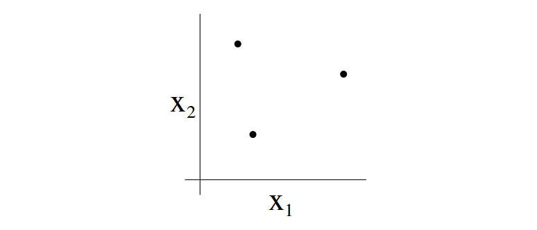
So assume that we have a hypothesis class in 2D, can this hypothesis class classify any possible labeling for these three points or shatter them? Given that $h(x) = \mathcal{1}\{\theta_0+\theta_1x_1+\theta_2x_2\}$, we can enumerate all possible labeling for these three points and draw a straight line in 2D to perfectly classify them. That is:

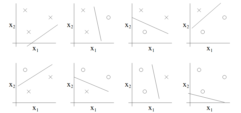
Moreover, we can prove that there is no set of 4 points that can be shattered by this hypothesis class. Thus, $VC(\mathcal{H})=3$.

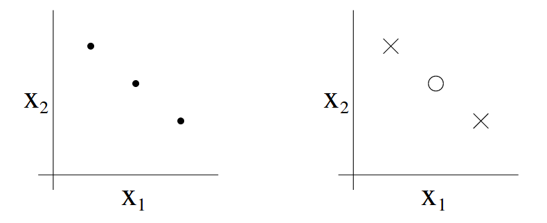
Note that not all possible of set of 3 points can be shattered by this hypothesis class even if VC dimension is 3. The below is an example for such as case where this hypothesis class failed to classify them.

Thus, to prove that some hypothesis class has VC dimension at least d, we just need to it can shatter at least one set of points with size d.

Theorem Let $\mathcal{H}$ be given and $d = VC(\mathcal{H})$. Then with porbability at least $1-\delta$, we have that for all $h\in\mathcal{H}$:

\[\lvert\varepsilon(h) - \lvert\hat{\varepsilon}(h)\rvert\leq O\bigg(\sqrt{\frac{d}{m}\log\frac{m}{d}+\frac{1}{m}\log\frac{1}{\delta}}\bigg)\]

Thus, with probabilyt at least $1-\delta$, we also have that:

\[\varepsilon(\hat{h}) \leq \varepsilon(h^{\ast}) + O\bigg(\sqrt{\frac{d}{m}\log\frac{m}{d}+\frac{1}{m}\log\frac{1}{\delta}}\bigg)\]

It means that if a hypothesis class has a finite VC dimension, the uniform convergence happens as m goes large. We use similar derivation from finite hypothesis class to give a bound on $\varepsilon(\hat{h})$ in terms of $\varepsilon(h^{\ast})$.

Corollary For $\lvert\varepsilon(h) - \hat{\lvert\varepsilon(h)}\rvert\leq\gamma$ to hold for all $h\in\mathcal{H}$ with probability at least $1-\delta$, it suffices that $m=O_{\gamma,\delta}(d)$ where d is the VC dimension.

In short, the number of training samples we need to train well using a particular $\mathcal{H}$ is linear in the VC dimension of $\mathcal{H}$. In general, VC dimension for most hypothesis classes is approximately linear in the number of parameters. So the number of needed traning samples is also related to the number of parameters.